Fivepoint Stencil Formula a Continuous Function

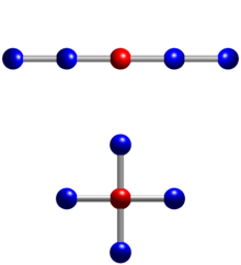
An illustration of the five-point stencil in one and two dimensions (top, and bottom, respectively).

In numerical analysis, given a square grid in one or two dimensions, the five-point stencil of a point in the grid is a stencil made up of the point itself together with its four "neighbors". It is used to write finite difference approximations to derivatives at grid points. It is an example for numerical differentiation.

In one dimension [edit]

In one dimension, if the spacing between points in the grid is h, then the five-point stencil of a point x in the grid is

${\displaystyle \ \{x-2h,x-h,x,x+h,x+2h\}.}$

1D first derivative [edit]

The first derivative of a function ƒ of a real variable at a point x can be approximated using a five-point stencil as:^[1]

${\displaystyle f'(x)\approx {\frac {-f(x+2h)+8f(x+h)-8f(x-h)+f(x-2h)}{12h}}}$

Notice that the center point ƒ(x) itself is not involved, only the four neighboring points.

Derivation [edit]

This formula can be obtained by writing out the four Taylor series of ƒ(x ±h) and ƒ(x ± 2h) up to terms of h ³ (or up to terms of h ⁵ to get an error estimation as well) and solving this system of four equations to get ƒ^′(x). Actually, we have at points x +h and x −h:

${\displaystyle f(x\pm h)=f(x)\pm hf'(x)+{\frac {h^{2}}{2}}f''(x)\pm {\frac {h^{3}}{6}}f^{(3)}(x)+O_{1\pm }(h^{4}).\qquad (E_{1\pm }).}$

Evaluating ${\displaystyle (E_{1+})-(E_{1-})}$ gives us

${\displaystyle f(x+h)-f(x-h)=2hf'(x)+{\frac {h^{3}}{3}}f^{(3)}(x)+O_{1}(h^{4}).\qquad (E_{1}).}$

Note that the residual term O₁(h ⁴) should be of the order of h ⁵ instead of h ⁴ because if the terms of h ⁴ had been written out in (E ₁₊) and (E ₁₋), it can be seen that they would have canceled each other out by ƒ(x +h) − ƒ(x −h). But for this calculation, it is left like that since the order of error estimation is not treated here (cf below).

Similarly, we have

${\displaystyle f(x\pm 2h)=f(x)\pm 2hf'(x)+{\frac {4h^{2}}{2!}}f''(x)\pm {\frac {8h^{3}}{3!}}f^{(3)}(x)+O_{2\pm }(h^{4}).\qquad (E_{2\pm })}$

and ${\displaystyle (E_{2+})-(E_{2-})}$ gives us

${\displaystyle f(x+2h)-f(x-2h)=4hf'(x)+{\frac {8h^{3}}{3}}f^{(3)}(x)+O_{2}(h^{4}).\qquad (E_{2}).}$

In order to eliminate the terms of ƒ⁽³⁾(x), calculate 8 × (E ₁) − (E ₂)

${\displaystyle 8f(x+h)-8f(x-h)-f(x+2h)+f(x-2h)=12hf'(x)+O(h^{4})\,}$

thus giving the formula as above. Note: the coefficients of f in this formula, (8, -8,-1,1), represent a specific example of the more general Savitzky–Golay filter.

Error estimate [edit]

The error in this approximation is of order h  ⁴. That can be seen from the expansion

${\displaystyle {\frac {-f(x+2h)+8f(x+h)-8f(x-h)+f(x-2h)}{12h}}=f'(x)-{\frac {1}{30}}f^{(5)}(x)h^{4}+O(h^{5})}$ ^[2]

which can be obtained by expanding the left-hand side in a Taylor series. Alternatively, apply Richardson extrapolation to the central difference approximation to ${\displaystyle f'(x)}$ on grids with spacing 2h and h.

1D higher-order derivatives [edit]

The centered difference formulas for five-point stencils approximating second, third, and fourth derivatives are

${\displaystyle f''(x)\approx {\frac {-f(x+2h)+16f(x+h)-30f(x)+16f(x-h)-f(x-2h)}{12h^{2}}}}$

${\displaystyle f^{(3)}(x)\approx {\frac {f(x+2h)-2f(x+h)+2f(x-h)-f(x-2h)}{2h^{3}}}}$

${\displaystyle f^{(4)}(x)\approx {\frac {f(x+2h)-4f(x+h)+6f(x)-4f(x-h)+f(x-2h)}{h^{4}}}}$

The errors in these approximations are O(h  ⁴), O(h  ²) and O(h  ²) respectively.^[2]

Relationship to Lagrange interpolating polynomials [edit]

As an alternative to deriving the finite difference weights from the Taylor series, they may be obtained by differentiating the Lagrange polynomials

${\displaystyle \ell _{j}(\xi )=\prod _{i=0,\,i\neq j}^{k}{\frac {\xi -x_{i}}{x_{j}-x_{i}}},}$

where the interpolation points are

${\displaystyle x_{0}=x-2h,\quad x_{1}=x-h,\quad x_{2}=x,\quad x_{3}=x+h,\quad x_{4}=x+2h.}$

Then, the quartic polynomial ${\displaystyle p_{4}(x)}$ interpolating ƒ(x) at these five points is

${\displaystyle p_{4}(x)=\sum \limits _{j=0}^{4}f(x_{j})\ell _{j}(x)}$

and its derivative is

${\displaystyle p_{4}'(x)=\sum \limits _{j=0}^{4}f(x_{j})\ell '_{j}(x).}$

So, the finite difference approximation of ƒ ^′(x) at the middle point x =x ₂ is

${\displaystyle f'(x_{2})=\ell _{0}'(x_{2})f(x_{0})+\ell _{1}'(x_{2})f(x_{1})+\ell _{2}'(x_{2})f(x_{2})+\ell _{3}'(x_{2})f(x_{3})+\ell _{4}'(x_{2})f(x_{4})+O(h^{4})}$

Evaluating the derivatives of the five Lagrange polynomials at x=x ₂ gives the same weights as above. This method can be more flexible as the extension to a non-uniform grid is quite straightforward.

In two dimensions [edit]

In two dimensions, if for example the size of the squares in the grid is h by h, the five point stencil of a point (x,y) in the grid is

${\displaystyle \{(x-h,y),(x,y),(x+h,y),(x,y-h),(x,y+h)\},\,}$

forming a pattern that is also called a quincunx. This stencil is often used to approximate the Laplacian of a function of two variables:

${\displaystyle \nabla ^{2}f(x,y)\approx {\frac {f(x-h,y)+f(x+h,y)+f(x,y-h)+f(x,y+h)-4f(x,y)}{h^{2}}}.}$

The error in this approximation is O(h  ²),^[3] which may be explained as follows:

From the 3 point stencils for the second derivative of a function with respect to x and y:

${\displaystyle {\begin{array}{l}{\frac {\partial ^{2}f}{\partial x^{2}}}={\frac {f\left(x+\Delta x,y\right)+f\left(x-\Delta x,y\right)-2f(x,y)}{\Delta x^{2}}}-2{\frac {f^{(4)}(x,y)}{4!}}\Delta x^{2}+\cdots \end{array}}}$

${\displaystyle {\begin{array}{l}{\frac {\partial ^{2}f}{\partial y^{2}}}={\frac {f\left(x,y+\Delta y\right)+f\left(x,y-\Delta y\right)-2f(x,y)}{\Delta y^{2}}}-2{\frac {f^{(4)}(x,y)}{4!}}\Delta y^{2}+\cdots \end{array}}}$

If we assume ${\displaystyle \Delta x=\Delta y=h}$ :

${\displaystyle {\begin{array}{ll}\nabla ^{2}f&={\frac {\partial ^{2}f}{\partial x^{2}}}+{\frac {\partial ^{2}f}{\partial y^{2}}}\\&={\frac {f\left(x+h,y\right)+f\left(x-h,y\right)+f\left(x,y+h\right)+f\left(x,y-h\right)-4f(x,y)}{h^{2}}}-4{\frac {f^{(4)}(x,y)}{4!}}h^{2}+\cdots \\&={\frac {f\left(x+h,y\right)+f\left(x-h,y\right)+f\left(x,y+h\right)+f\left(x,y-h\right)-4f(x,y)}{h^{2}}}+O\left(h^{2}\right)\\\end{array}}}$

See also [edit]

• Stencil jumping
• Finite difference coefficients
• Iterative Stencil Loops

References [edit]

1. ^ Sauer, Timothy (2012). Numerical Analysis. Pearson. p. 250. ISBN978-0-321-78367-7.
2. ^ ^{a b} Abramowitz & Stegun, Table 25.2
3. ^ Abramowitz & Stegun, 25.3.30

• Abramowitz, Milton; Stegun, Irene A. (1970), Handbook of Mathematical Functions with Formulas, Graphs, and Mathematical Tables, Dover . Ninth printing. Table 25.2.

davisversely.blogspot.com

Source: https://en.wikipedia.org/wiki/Five-point_stencil

Share this post